I wrote this material for a digital signals processing assignment in fourth year university. I am re-posting it here in response to a Stack Exchange question.

The FFT in 30 seconds…

The Discrete Fourier Transform (DFT) takes a piece of a signal of interest, length N samples, assumes a periodic extension of the signal to infinity in both directions, and decomposes that periodic signal into a sum of N discrete frequency components.

The frequencies analysed are harmonics of the original signal length, T, which becomes the period length of the periodic extension of the signal. The DFT finds a magnitude and a phase for each of the frequency components (or ‘bins’.)

The Fast Fourier Transform, or FFT, is an efficient recursive algorithm for implementing the DFT with O (n log n) running time (instead of O(n²) for naive implementations of the DFT.)

Vanilla FFT

In this example, we will sample a 70Hz cosine wave for one second, at a rate 256 samples/sec. This will yield a discrete sequence of length 256, which we may analyse using the FFT.

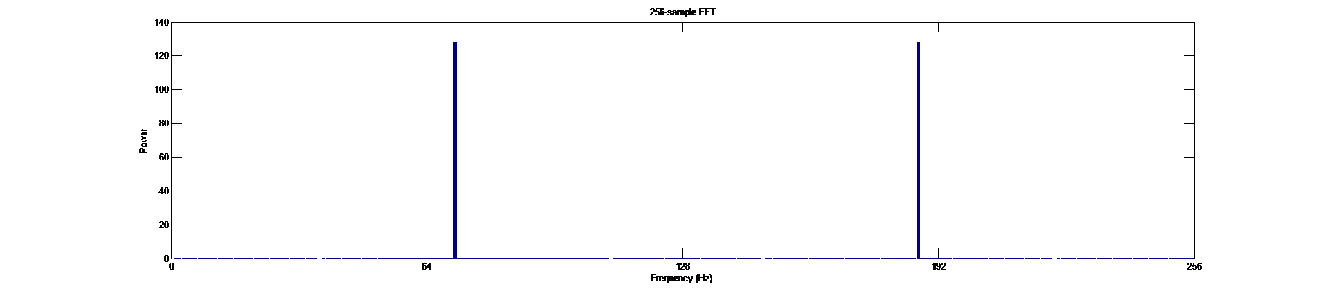
As we can see, the FFT correctly determines that the original signal was a 70Hz sinusoid. Note that since our sample of the signal captured an integer number of the sinusoid’s cycles, the original frequency was resolved perfectly.

It is also noteworthy that we sampled the original signal at 256Hz; therefore, the spectrum is symmetrical around the Nyquist rate of 128Hz. (Footnote 1)

Sequence padding to increase FFT resolution

Sometimes we desire to increase the resolution of the FFT - that is, how finely the frequency samples are spaced between zero and the sampling frequency.

One way to do this is to pad the time sequence with zeroes, making it a longer sequence. Since the FFT puts the signal into as many frequency bins as there are signal samples, doubling the length of the time signal by zero padding will also double the number of frequency bins, in the same frequency span.

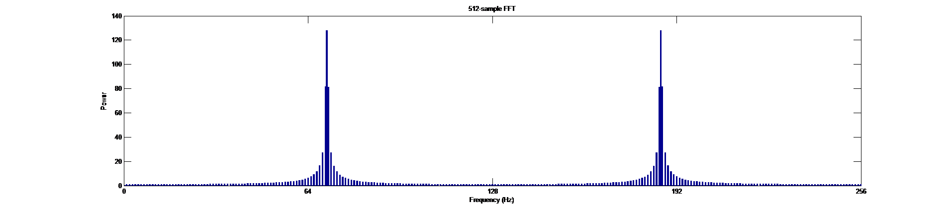
When we implement this, we get an unpleasant surprise; the signal power we should be seeing at 70Hz only has ‘leaked’ into the bins adjacent to it. This effect is called ‘spectral leakage’ and is due to the zero padding of the original sequence. To get a better look at what is happening, we zero pad the sequence to 64 times original length and have a closer look at what pattern emerges around the original 70hz spectral component.

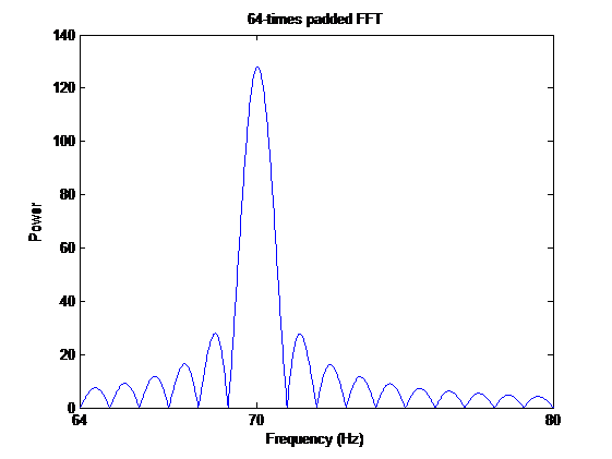
It looks as if the original spike at 70Hz has been replaced by a sinc(f) centred on the same spot. Why?

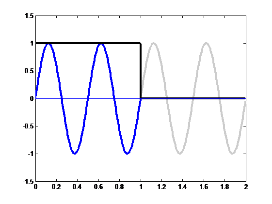
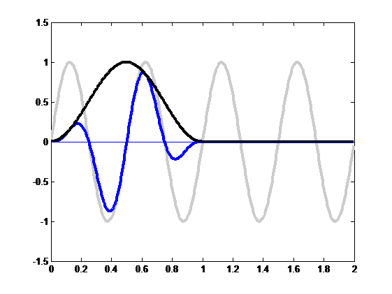
When we zero-pad the time sequence, we effectively extend it to twice the length, then multiply it by a rectangular window; we then want to take the periodic extension of this enlarged signal and find the FFT.

We illustrate this above; we have extended the signal to double the usual length (the gray line) and then multiplied it by a rectangular window (black line) to give the zero-padded signal, the blue line.

The problem lies in that multiplying the original signal with the rectangular window is equivalent to convolving the spectra of the original signal (an impulse at 70Hz) with the spectra of the rectangular window. Since the spectrum of the rectangular window is the sinc(x) function, we observe the characteristic sin(x)/x lobes around each of our original spectral components as they are convolved with the window spectrum.

Windowing + Zero Padding = Less leakage

If we extend the signal by repeating the sequence we already had (instead of naively zero-padding it), we could obtain increased resolution without any spectral leakage. However, this may be more computationally expensive to do in practice, so we seek a method that will let us zero-pad our signal – a cheap operation – but reduce the effects of spectral leakage.

The main issue with naive zero-padding is that it amounts to convolution of the original spectrum (which we would like to obtain with high fidelity) with the spectrum of a rectangular window, which has a sin(x)/x envelope and thus smears the original spectrum very severely.

However, we can choose a window functions other than the rectangular window with tighter-grouped (less ‘smeary’) spectral representations. When the signal spectrum is convolved with this tighter window spectrum, less smearing results.

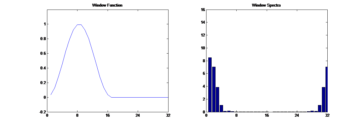
One such window is the Hann window (a.k.a. the Hanning window), which is shaped like half a sinusoid cycle. Its shape and spectra are illustrated above.

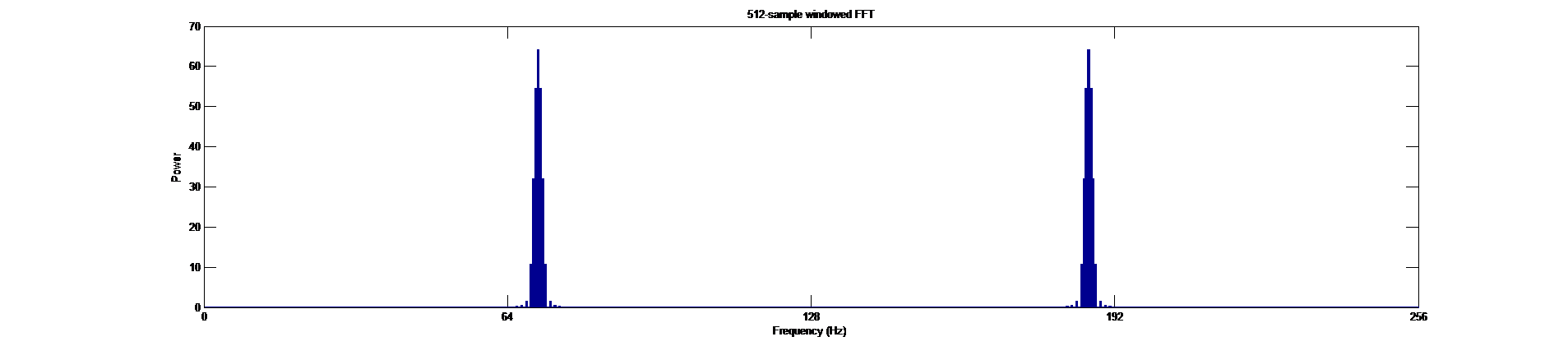
When we apply the Hann window to the data and then zero pad, we obtain a data sequence that ‘tapers off to zero’ at the ends, as opposed to rectangular windowing (which is a sharp transition.) The FFT for the Hann-windowed and padded sequence is shown above; we see that there is far less smearing of the spectral components than before.

Comments

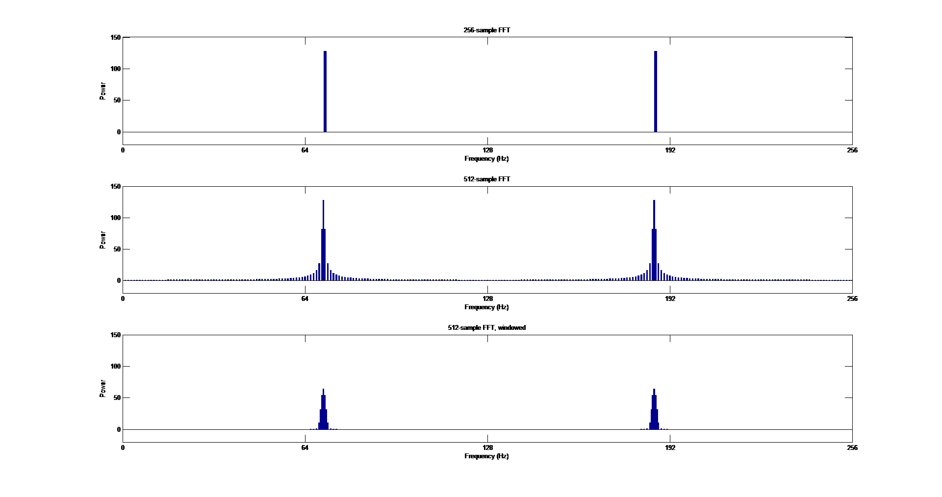
From top to bottom, the figure above reproduces the spectral plots for

1. the non-extended sequence
2. the naively zero-padded (rectangular windowed) extended sequence
3. the zero-padded and Hann windowed extended sequence.

When we want to increase the resolution of the FFT by zero-padding, clearly we would like the higher-resolution FFT to resemble the original spectrum as much as possible. We have a choice of window functions we can apply to the data before zero-padding; these will influence the character of the higher-resolution FFT.

In this example, we would clearly prefer the Hann window to the rectangular window, because there is only one spectral component in the original signal (and we would like to resolve this to the best accuracy.)

However, the choice of window is not always so clear-cut (Footnote 2). The choice of window is a compromise between ability to resolve finely-spaced frequency components (resolution) and ability to detect small signals near to large signals (dynamic range).

It turns out that the rectangular window has poor dynamic range - because there is a lot of out-of-band power in its spectrum – but it has excellent resolution, because the main lobe is very tall compared to the side lobes. It is actually useful when the main criteria is detecting closely-spaced spectral components.

Footnote 1: Note to self: What happens when we have signals in quadrature, as per QAM modulation? Must investigate the FFT of quadrature-encoded signals in MATLAB – is the spectrum still symmetrical around the Nyquist frequency?

Footnote 2: Wikipedia: Window Function has an enlightening discussion on choice of windows.